Independent Component Analysis

25 August 2021

It feels like something like independent component analysis (ICA) would be important for unsupervised learning, especially with recent advances in non-linear ICA (e.g. here or here; also see this overview talk). Here I’d like to simply learn the basics of ICA. Independently, I’d like to learn the basics of Jax, a source-to-source autodiff system.

I’m going to implement a basic version of gradient-based maximum likelihood estimation of an ICA model. To learn about this, I’ve used the following resources

Generative model

In a simplified ICA, we assume there are \(N\) signals \(x_{1:N}\) and \(N\) sources \(z_{1:N}\), and that each signal \(x_n\) and each source \(z_n\) is \(D\)-dimensional. Given a mixing matrix \(W \in \mathbb R^{D \times D}\) which we will want to learn, the generative model is \begin{align} z_n &\sim p_z(z_n) = \prod_{d = 1}^D p_{z_d}(z_{nd}) \\
x_n &= W z_n. \end{align} It’s important that the components of \(z_n\) are independent and that \(p_{z_d}\) is not Gaussian. In practice, \(p_z\) is just set to \(\log \cosh\) or square root depending on whether the signal is supergaussian or subgaussian.

Maximum likelihood estimation

The goal here is to estimate \(W\) using maximum likelihood \begin{align} W^* = \argmax_W p(x_{1:N} | W). \end{align}

This might seem hard because of the required marginalization over \(z_{1:N}\) but since we’re just assuming a noise-free mapping from source to signal, we can just use the change-of-variable identity to get \begin{align} p(x_n) = p_z(W^{-1} x_n) |\det (W^{-1}) |. \end{align}

Letting \(V = W^{-1}\), we can write the loss as the average of the likelihood terms over all \(N\) signals \begin{align} \mathcal L(V) = \frac{1}{N} \sum_{n = 1}^N (-\log p_z(Vx_n) - \log |\det V|). \end{align}

For supergaussian components we should choose a supergaussian prior \(p_z\) and for subgaussian data we should choose a subgaussian prior \(p_z\). It doesn’t actually matter which prior exactly. As long as we identify sub/super-gaussianity, we should be good.

Simplifying the problem further by preprocessing the data

To further simplify the learning, assume that \(z_{nd}\) and \(x_{nd}\) are zero mean and unit variance. The former can be achieved by setting appropriate priors and the latter by centering and whitening the data before running the algorithm. What this also achieves though is that \(W\) (and thus \(V\)) are orthogonal matrices since \begin{align} \Cov[x_n]= \E[x_n x_n^T] = \E[Wz_n z_n^T W^T] = W \E[z_n z_n^T] W^T = WW^T = I. \end{align} Since the determinant of an orthogonal matrix is \(\pm 1\), we can drop the log determinant term from the loss \begin{align} \mathcal L(V) = \frac{1}{N} \sum_{n = 1}^N -\log p_z(Vx_n). \label{eq:loss} \end{align} We also only need \(D (D - 1) / 2\) parameters to parameterize a \(D\)-by-\(D\) orthogonal matrix (e.g. using Cayley’s transform).

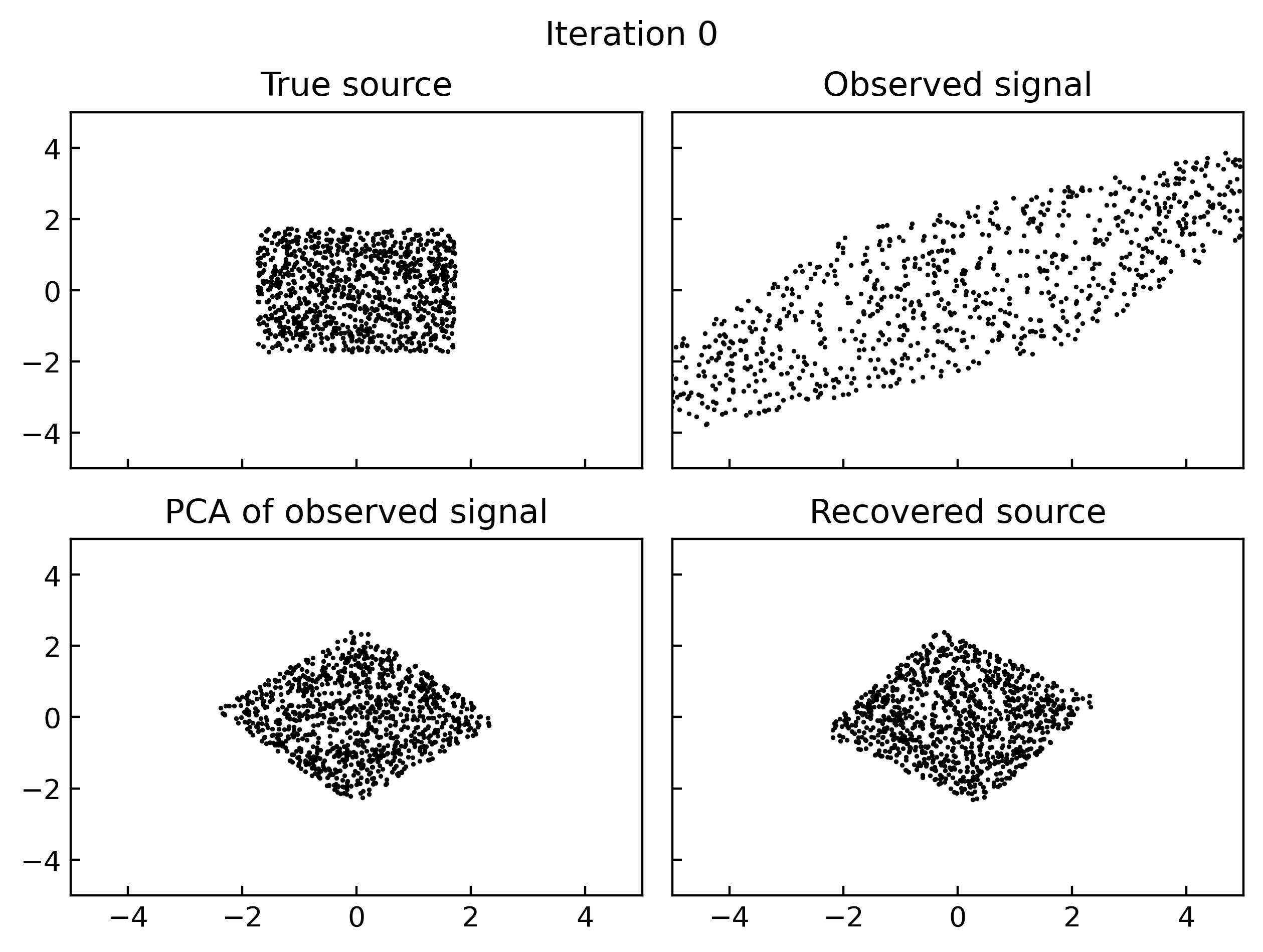
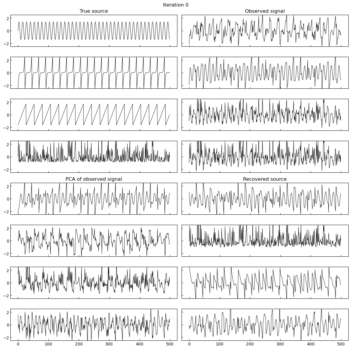
Results

A simple implementation of gradient based maximum likelihood estimation of ICA in Jax, which produces the following gifs can be found here.

Why do I think this works?

(I’m just playing around/exploring below. See Section 4 of Aapo Hyvärinen’s and Erkki Oja’s tutorial for a proper explanation.)

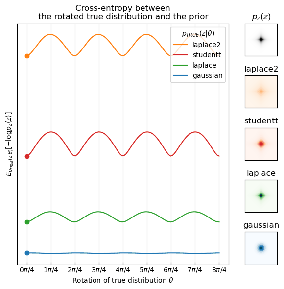
Given the loss in \eqref{eq:loss}, the choice of the prior \(p_z\) seems to be very important. As mentioned before, as long as we know whether the components are subgaussian or supergaussian, we can just the prior \(p_z\) to be from the same family and minimizing the loss should yield the “correct” mixing matrix. And if the components are gaussian, we can’t find the mixing matrix anyway. How come?

The loss can actually be reinterpreted as an approximation of the cross-entropy between the true distribution of the components \(p_{\text{TRUE}}(z)\)—in our case this would be whatever the distribution of \(Vx_n\) is—and the prior \(p_z(z)\) \begin{align} \mathcal L \approx H(p_{\text{TRUE}}(z), p_z(z)) = \E_{p_{\text{TRUE}}(z)}[-\log p_z(z)]. \end{align}

It turns out however, that if \(p_{\text{TRUE}}\) and \(p_z\) are both supergaussian or both subgaussian, the cross-entropy is the lowest at the “correct rotations” of \(p_{\text{TRUE}}\). Below, I visualize this in 2D. Fix the prior \(p_z\) to be a supergaussian distribution, in this case standard laplace, and look at different true distributions \(p_{\text{TRUE}}(z | \theta)\) rotated by an angle \(\theta \in [0, 2\pi]\). The cross-entropy is minimized at 90-degree multiples if \(p_{\text{TRUE}} = p_z\) but also for any other supergaussian distribution (laplace with higher standard deviation or student T). For a gaussian \(p_{\text{TRUE}}\), the cross-entropy is constant which implies that we can’t find the “correct rotation” by minimizing the cross-entropy.

[back]