Tuan Anh Le
gaussian processes for regression
20 June 2017
these notes follow chapter 2 of the gp book (Rasmussen & Williams, 2006) and the tutorial (Rasmussen, 2004).
let \((x_n, y_n)_{n = 1}^N, x_n \in \mathcal X, y_n \in \mathbb R\) be data. our goal is to predict \(y_\ast\) for a new input \(x_\ast \in \mathcal X\) (possibly predict multiple outputs given multiple inputs).
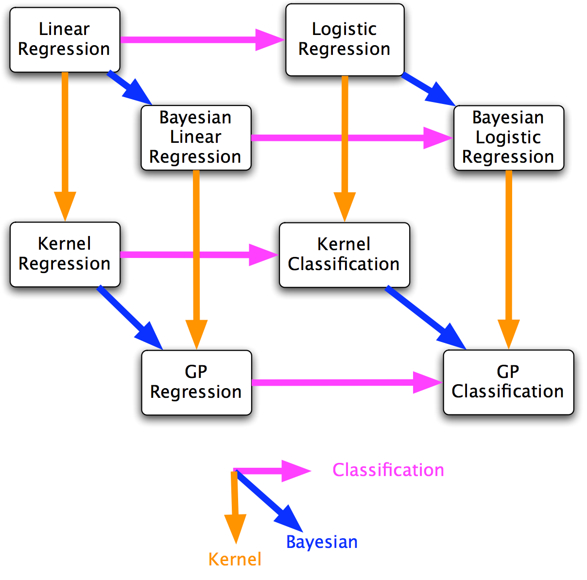
we summarize two views. the weight-space view develops gp regression by extending bayesian linear regression. the function-space view develops the same by viewing gps as distribution over functions.
referring to zoubin’s cube below, the weight-space view starts from bayesian linear regression and follows the downward arrow to obtain gp regression. the function-space view, on the other hand, directly tackles gp regression. the latter is the real deal.
weight-space view
bayesian linear regression
define
- feature mapping \(\phi: \mathcal X \to \mathbb R^D\),
- features \(\phi_n := \phi(x_n), n = 1, \dotsc, N\),
- \(\phi_\ast := \phi(x_\ast)\),
- feature matrix \(\Phi := [\phi_1, \dotsc, \phi_N]^T \in \mathbb R^{N \times D}\),
- inputs \(x := \{x_1, \dotsc, x_N\}\),
- outputs \(y := [y_1, \dotsc, y_N]^T \in \mathbb R^D\),
- weights \(w \in \mathbb R^D\).
let the generative model be
\begin{align}
p(w) &= \mathrm{Normal}(w; 0, \Sigma), \\
p(y \given x, w) &= \mathrm{Normal}(y; \Phi w, \sigma^2 I),
\end{align}
where \(0\) is a zero vector and \(I\) is an identity matrix of suitable dimensions, \(\Sigma \in \mathbb R^{D \times D}\) is the prior covariance matrix, \(\sigma^2 > 0\) is the observation noise variance.
the posterior over weights is (via completing the square)
\begin{align}
p(w \given x, y) &= \frac{p(y \given x, w) p(w)}{p(y \given x)} \\
&= \mathrm{Normal}(w; m, S) \\
m &= S \cdot \left(\frac{1}{\sigma^2} \Phi^T y\right) \\
S &= \left(\Sigma^{-1} + \frac{1}{\sigma^2} \Phi^T \Phi\right)^{-1}.
\end{align}
the posterior predictive is (via equation 5 of michael osborne’s note)
\begin{align}
p(y_\ast \given x_\ast, x, y) &= \int p(y_\ast \given x_\ast) p(w \given x, y) \,\mathrm dw \\
&= \mathrm{Normal}(y_\ast \given \phi_\ast^T m, \sigma^2 + \phi_\ast^T S \phi_\ast).
\end{align}
the marginal likelihood is (via equation 5 of michael osborne’s note)
\begin{align}
p(y \given x) &= \int p(y \given x, w) p(w) \,\mathrm dw \\
&= \mathrm{Normal}(y \given 0, \sigma^2 I + \Phi \Sigma \Phi^T) \\
&= (2\pi)^{-N/2} \cdot \mathrm{det}(\sigma^2 I + \Phi \Sigma \Phi^T)^{-1/2} \cdot \exp\left(-\frac{1}{2} y^T (\sigma^2 I + \Phi \Sigma \Phi^T)^{-1} y \right). \label{eq:gp-regression/bayesian-linear-regression-marginal-likelihood}
\end{align}
bayesian linear regression to gp regression
we can rewrite the posterior predictive (using matrix inversion lemmas described on page 12 of (Rasmussen & Williams, 2006))
\begin{align}
p(y_\ast \given x_\ast, x, y) &= \mathrm{Normal}(y_\ast \given \phi_\ast^T m, \sigma^2 + \phi_\ast^T S \phi_\ast) \\
&= \mathrm{Normal}(y_\ast \given \color{red}{\phi_\ast^T \Sigma \Phi^T} (\color{blue}{\Phi \Sigma \Phi^T} + \sigma^2 I)^{-1} y, \color{green}{\phi_\ast^T \Sigma \phi_\ast} - \color{red}{\phi_\ast^T \Sigma \Phi^T} (\color{blue}{\Phi \Sigma \Phi^T} + \sigma^2 I)^{-1} \color{red}{\Phi \Sigma \phi_\ast} ), \\
&= \mathrm{Normal}(y_\ast \given \color{red}{k_\ast^T} (\color{blue}{K} + \sigma^2 I)^{-1} y, \color{green}{k_{\ast \ast}} - \color{red}{k_\ast^T} (\color{blue}{K} + \sigma^2 I)^{-1} \color{red}{k_\ast} ), \label{eq:gp-regression/bayesian-linear-regression-prediction} \\
\color{blue}{K} &:= \color{blue}{\Phi \Sigma \Phi^T}, \\
\color{red}{k_\ast} &:= \color{red}{\Phi \Sigma \phi_\ast}, \\
\color{green}{k_{\ast \ast}} &:= \color{green}{\phi_\ast^T \Sigma \phi_\ast}.
\end{align}
similarly, we can rewrite the marginal likelihood \begin{align} p(y \given x) &= (2\pi)^{-N/2} \cdot \mathrm{det}(\sigma^2 I + \color{blue}{K})^{-1/2} \cdot \exp\left(-\frac{1}{2} y^T (\sigma^2 I + \color{blue}{K})^{-1} y \right). \end{align}
define a kernel (or covariance) function \(k: \mathcal X \times \mathcal X \to \mathbb R\): \begin{align} k(x, x’) := \phi(x)^T \Sigma \phi(x’), \forall x, x’ \in \mathcal X. \end{align} hence, if we can evaluate \(k\), we can obtain \(\color{blue}{K}, \color{red}{k_\ast}, \color{green}{k_{\ast \ast}}\) without having to do the matrix multiplications. this is exactly what we do in zero-mean gp regression: we specify a kernel function \(k\) using which we can do prediction and evaluate marginal likelihood. see kernel literature for why choosing a positive semidefinite kernel function \(k\) implies existence of feature map \(\phi\). for example, it can be shown that the exponentiated-square kernel function corresponds to bayesian linear regression model with an infinite number of basis functions. using \(k\) instead of performing matrix multiplications is sometimes called kernel trick.
function-space view
this section heavily follows (Rasmussen, 2004).
gaussian process
definition (gaussian process). a gaussian process is a collection of random variables, any finite number of which have consistent joint normal distributions.
the collection of random variables is indexed by \(\mathcal X\) which can be arbitrary. a random variable in this collection indexed by \(x \in \mathcal X\) is denoted \(f(x)\) (instead of \(f_x\)).
consider an arbitrary, finite number \(N\), of random variables from the gaussian process, \((f(x_1), \dotsc, f(x_N)), x_n \in \mathcal X\) (note that the indices \(n\) don’t imply any ordering other than notational convenience. \(x_n\) are the indices of the gaussian process!). by definition, \((f(x_1), \dotsc, f(x_N))\) has a multivariate normal distribution, say \(\mathrm{Normal}(\mu, \Sigma)\).
the consistent part means that any subset of \((f(x_1), \dotsc, f(x_N))\) has a multivariate normal distribution \(\mathrm{Normal}(\mu', \Sigma')\) where \(\mu', \Sigma'\) are the corresponding sub-entries of \(\mu, \Sigma\).
a gp is specified by its mean function \(m: \mathcal X \to \mathbb R\) and covariance function \(k: \mathcal X \times \mathcal X \to \mathbb R\). we consider a gp to be a distribution over functions and write \begin{align} f \sim \mathcal{GP}(m, k). \end{align}
the mean and covariance functions specify fully the distribution of \(f\) at any finite number \(N\) of indices \(x_n \in \mathcal X, n = 1, \dotsc, N\):
\begin{align}
(f(x_1), \dotsc, f(x_N)) \sim \mathrm{Normal}\left(
\begin{bmatrix}
m(x_1) \\
\vdots \\
m(x_N)
\end{bmatrix},
\begin{bmatrix}
k(x_1, x_1) & \dots & k(x_1, x_N) \\
\vdots & \ddots & \vdots \\
k(x_N, x_1) & \dots & k(x_N, x_N)
\end{bmatrix}
\right).
\end{align}
we can also see (by inspection) that the consistency criterion is satisfied.
posterior gaussian process
if we condition on a finite number \(N\) random variables of the gp \(f\), \(f(x_1), \dotsc, f(x_N)\), we also obtain a gp which we call the posterior gp.
to this end, let
\begin{align}
\vec f &:= [f(x_1), \dotsc, f(x_N)]^T \\
\vec f_\ast &:= [f(x_{1, \ast}), \dotsc, f(x_{M, \ast})]^T,
\end{align}
where \(\vec f\) are the random variables we condition on and \(\vec f_\ast\) are \(M\) random variables at indices \(x_{m, \ast} \in \mathcal X\).
we have
\begin{align}
\begin{bmatrix}
\vec f \\
\vec f_\ast
\end{bmatrix} &\sim
\mathrm{Normal}\left(
\begin{bmatrix}
\vec \mu \\
\vec \mu_\ast
\end{bmatrix},
\begin{bmatrix}
\Sigma & \Sigma_\ast \\
\Sigma_\ast^T & \Sigma_{\ast\ast}
\end{bmatrix}
\right), \\
\vec \mu &:= [m(x_1), \dotsc, m(x_N)]^T, \\
\vec \mu_\ast &:= [m(x_{1, \ast}), \dotsc, m(x_{M, \ast})]^T, \\
\Sigma &:= \begin{bmatrix}
k(x_1, x_1) & \dots & k(x_1, x_N) \\
\vdots & \ddots & \vdots \\
k(x_N, x_1) & \dots & k(x_N, x_N)
\end{bmatrix}, \\
\Sigma_\ast &:= \begin{bmatrix}
k(x_1, x_{1, \ast}) & \dots & k(x_1, x_{M, \ast}) \\
\vdots & \ddots & \vdots \\
k(x_N, x_{1, \ast}) & \dots & k(x_N, x_{M, \ast})
\end{bmatrix}, \\
\Sigma_{\ast\ast} &:= \begin{bmatrix}
k(x_1, x_1) & \dots & k(x_1, x_{M, \ast}) \\
\vdots & \ddots & \vdots \\
k(x_{M, \ast}, x_1) & \dots & k(x_{M, \ast}, x_{M, \ast})
\end{bmatrix}.
\end{align}
using equation 2 in michael osborne’s note, we obtain \begin{align} \vec f_\ast \given \vec f &\sim \mathrm{Normal}\left(\vec \mu_\ast + \Sigma_\ast^T \Sigma^{-1} (\vec f - \vec \mu), \Sigma_{\ast \ast} - \Sigma_\ast^T \Sigma^{-1} \Sigma_\ast\right). \label{eq:gp-regression/finite-posterior} \end{align}
by inspection,
\begin{align}
f \given f(x_1), \dotsc, f(x_N) &\sim \mathcal{GP}(m_{\text{posterior}}, k_{\text{posterior}}), \\
m_{\text{posterior}}(x) &:= m(x) + \Sigma_{\ast, x}^T \Sigma^{-1} (\vec f - \vec \mu), \\
k_{\text{posterior}}(x, x’) &:= k(x, x’) - \Sigma_{\ast, x}^T \Sigma^{-1} \Sigma_{\ast, x’}, \\
\Sigma_{\ast, x} &:= [k(x_1, x), \dotsc, k(x_N, x)]^T.
\end{align}
this is true by inspection in the sense that the distribution of \(M\) arbitrary random variables \(x_{1, \ast}, \dotsc, x_{M, \ast}\) from this process is a multivariate normal distribution given in \eqref{eq:gp-regression/finite-posterior}, i.e.
\begin{align}
\begin{bmatrix}
m_{\text{posterior}}(x_{1, \ast}) \\
\vdots \\
m_{\text{posterior}}(x_{M, \ast})
\end{bmatrix} &= \vec \mu_\ast + \Sigma_\ast^T \Sigma^{-1} (\vec f - \vec \mu), \\
\begin{bmatrix}
k_{\text{posterior}}(x_{1, \ast}, x_{1, \ast}) & \dots & k_{\text{posterior}}(x_{1, \ast}, x_{M, \ast}) \\
\vdots & \ddots & \vdots \\
k_{\text{posterior}}(x_{M, \ast}, x_{1, \ast}) & \dots & k_{\text{posterior}}(x_{M, \ast}, x_{M, \ast})
\end{bmatrix} &= \Sigma_{\ast \ast} - \Sigma_\ast^T \Sigma^{-1} \Sigma_\ast.
\end{align}
noisy observations
consider the case when the points we observe are noisy observations of the gp at indices \(x_1, \dotsc, x_N\), i.e. \begin{align} y_n = f(x_n) + \epsilon_n, && \epsilon_n \sim \mathrm{Normal}(0, \sigma^2), n = 1, \dotsc, N. \end{align}
let
\begin{align}
\vec y &:= [y_1, \dotsc, y_N]^T \\
\vec \epsilon &:= [\epsilon_1, \dotsc, \epsilon_N]^T.
\end{align}
we have
\begin{align}
\begin{bmatrix}
\vec y \\
\vec f_\ast
\end{bmatrix} &=
\begin{bmatrix}
\vec f \\
\vec f_\ast
\end{bmatrix} +
\begin{bmatrix}
\vec \epsilon \\
0
\end{bmatrix}.
\end{align}
now we have to use some property of multivariate normal distributions (which one?) to obtain
\begin{align}
\begin{bmatrix}
\vec y \\
\vec f_\ast
\end{bmatrix} &\sim
\mathrm{Normal}\left(
\begin{bmatrix}
\vec \mu \\
\vec \mu_\ast
\end{bmatrix},
\begin{bmatrix}
\Sigma + \sigma^2 I & \Sigma_\ast \\
\Sigma_\ast^T & \Sigma_{\ast\ast}
\end{bmatrix}
\right). \label{eq:gp-regression/joint-noise}
\end{align}
using the same line as before, we obtain
\begin{align}
\vec f_\ast \given \vec y &\sim \mathrm{Normal}\left(\vec \mu_\ast + \Sigma_\ast^T (\Sigma + \sigma^2 I)^{-1} (\vec f - \vec \mu), \Sigma_{\ast \ast} - \Sigma_\ast^T (\Sigma + \sigma^2 I)^{-1} \Sigma_\ast\right). \label{eq:gp-regression/finite-posterior-noisy}
\end{align}
and
\begin{align}
f \given \vec y &\sim \mathcal{GP}(m_{\text{posterior (noisy)}}, k_{\text{posterior (noisy)}}), \\
m_{\text{posterior (noisy)}}(x) &:= m(x) + \Sigma_{\ast, x}^T (\Sigma + \sigma^2 I)^{-1} (\vec f - \vec \mu), \\
k_{\text{posterior (noisy)}}(x, x’) &:= k(x, x’) - \Sigma_{\ast, x}^T (\Sigma + \sigma^2 I)^{-1} \Sigma_{\ast, x’}.
\end{align}
if \(m \equiv 0\), the distribution of this gp at one test index \(x_\ast\) corresponds to the predictive distribution of bayesian linear regression in \eqref{eq:gp-regression/bayesian-linear-regression-prediction}.
gp learning
usually, the mean and covariance functions of a gp will have hyperparameters \(\theta\). ideally, we want to perform inference to obtain \(p(\theta \given \vec y)\), marginalizing out \(f\). first we need the marginal likelihood \(p(\vec y \given \theta)\).
marginal likelihood
we will ignore the hyperparameters \(\theta\) in this section.
first, note that equation \eqref{eq:gp-regression/joint-noise} implies another gp over \(f_{\text{noisy}}\):
\begin{align}
f_{\text{noisy}} &\sim \mathcal{GP}(m_{\text{noisy}}, k_{\text{noisy}}) \\
m_{\text{noisy}} &\equiv m \\
k_{\text{noisy}}(x, x’) &:=
\begin{cases}
k(x, x’) + \sigma^2 & \text{if } x \equiv x’ \equiv x_n \text{ for some } n \\
k(x, x’) & \text{otherwise}
\end{cases}.
\end{align}
hence, by the marginalization property of a gp,
\begin{align}
p(\vec y) &= \mathrm{Normal}(\vec y \given \vec \mu, \sigma^2 I + \Sigma) \\
&= (2\pi)^{-N/2} \cdot \mathrm{det}(\sigma^2 I + \Sigma)^{-1/2} \cdot \exp\left(-\frac{1}{2} (\vec y - \vec \mu)^T (\sigma^2 I + \Sigma)^{-1} (\vec y - \vec \mu) \right). \label{eq:gp-regression/gp-marginal-likelihood}
\end{align}
for \(m \equiv 0\), this corresponds to the marginal likelihood of bayesian linear regression in \eqref{eq:gp-regression/bayesian-linear-regression-marginal-likelihood}.
inference
to obtain \(p(\theta \given \vec y)\), we place a prior on \(\theta\) and use the gp marginal likelihood \eqref{eq:gp-regression/gp-marginal-likelihood} as the likelihood: \begin{align} p(\theta \given \vec y) &\propto p(\theta) p(\vec y \given \theta). \end{align}
optimization
or we can just optimize \(p(\vec y \given \theta)\) from \eqref{eq:gp-regression/gp-marginal-likelihood} directly using gradient methods.
References
- Rasmussen, C., & Williams, C. (2006). Gaussian Processes for Machine Learning. In Gaussian Processes for Machine Learning. MIT Press.
@book{rasmussen2006gaussian, title = {Gaussian Processes for Machine Learning}, author = {Rasmussen, Carl and Williams, Chris}, journal = {Gaussian Processes for Machine Learning}, year = {2006}, publisher = {MIT Press} } - Rasmussen, C. E. (2004). Gaussian processes in machine learning. In Advanced lectures on machine learning (pp. 63–71). Springer.
@incollection{rasmussen2004gaussian,
  title = {Gaussian processes in machine learning},
  author = {Rasmussen, Carl Edward},
  booktitle = {Advanced lectures on machine learning},
  pages = {63--71},
  year = {2004},
  publisher = {Springer}
}
[back]