REBAR and RELAX

26 December 2017

These are notes on the REBAR and RELAX papers.

Goal

Given Bernoulli random variable \(b \sim \mathrm{Bernoulli}(\theta)\) and a function \(f: \{0, 1\} \to \mathbb R\), estimate \begin{align} \frac{\partial}{\partial \theta} \E[f(b)]. \end{align}

Setup

Using \(p\) to denote both distributions and corresponding densities, let: \begin{align} u &\sim \mathrm{Uniform}(0, 1) = p^u \\
v &\sim \mathrm{Uniform}(0, 1) = p^v \\
z &= g(u, \theta) \sim p_\theta^z \label{eq:z} \\
b &\sim \mathrm{Bernoulli}(\theta) = p_\theta^b \\
b \given z &= H(z) \sim p^{b \given z} \\
z \given b &= \tilde g(v, \theta, b) \sim p_\theta^{z \given b}, \label{eq:z-given-b} \end{align} where \begin{align} g(u, \theta) &= \log \frac{\theta}{1 - \theta} + \log \frac{u}{1 - u} \\
H(z) &= \begin{cases} 1 & \text{ if } z \geq 0 \\
0 & \text{ otherwise} \end{cases} \\
\tilde g(v, \theta, b) &= \begin{cases} \log \left(\frac{v}{1 - v} \frac{1}{1 - \theta} + 1\right) & \text{ if } b = 1 \\
-\log \left(\frac{v}{1 - v}\frac{1}{\theta} + 1\right) & \text{ if } b = 0 \end{cases} \\
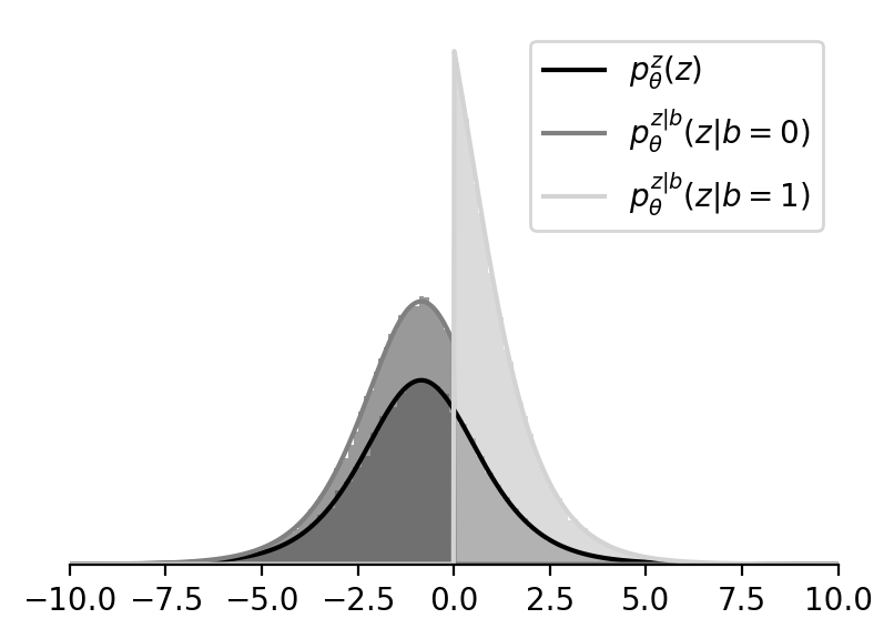
p_\theta^z(z) &= \frac{\frac{\theta}{1 - \theta} \exp(-z)}{\left(1 + \frac{\theta}{1 - \theta} \exp(-z)\right)^2} \\
p_\theta^{z \given b}(z \given b) &= \begin{cases} \frac{1}{\theta} \cdot p_\theta^z(z) \cdot H(z) & \text{ if } b = 1 \\
\frac{1}{1 - \theta} \cdot p_\theta^z(z) \cdot (1 - H(z)) & \text{ if } b = 0 \end{cases} \\
p^{b \given z}(b \given z) &= \begin{cases} \mathrm{Bernoulli(b; 1)} & \text{ if } z \geq 0 \\
\mathrm{Bernoulli(b; 0)} & \text{ if } z < 0. \end{cases} \end{align}

Properties: \begin{align} p_\theta^b(b) p_\theta^{z \given b}(z \given b) &= p_\theta^z(z) p^{b \given z}(b \given z) =: p_\theta^{z, b}(z, b) \\
p_\theta^b(b) &= \int p_\theta^{z, b}(z, b) \,\mathrm dz \\
p_\theta^z(z) &= \int p_\theta^{z, b}(z, b) \,\mathrm db. \end{align}

Plots:

Python script for generating these figures.

Derivation

\begin{align} \frac{\partial}{\partial \theta} \E_{p_\theta^b(b)}[f(b)] &= \frac{\partial}{\partial \theta} \E_{p_\theta^b(b) p_\theta^{z \given b}(z \given b)}[f(b)] & \text{(from Properties)} \\
&= \frac{\partial}{\partial \theta} \E_{p_\theta^b(b) p_\theta^{z \given b}(z \given b)}[f(b) - c(z) + c(z)]. \label{eq:derivation1} \end{align}

First term: \begin{align} \frac{\partial}{\partial \theta} \E_{p_\theta^b(b) p_\theta^{z \given b}(z \given b)}[f(b)] &= \frac{\partial}{\partial \theta} \E_{p_\theta^b(b)}[f(b)] & \text{(from Properties)} \\
&= \E_{p_\theta^b(b)}\left[f(b) \frac{\partial}{\partial \theta} \log p_\theta^b(b)\right] & \text{(REINFORCE trick)} \\
&= \E_{p^u(u)} \left[f(H(g(u, \theta))) \frac{\partial}{\partial \theta} \log p_\theta^b(H(g(u, \theta))) \right] & \text{(reparameterization)}. \end{align}

Second term: \begin{align} \frac{\partial}{\partial \theta} \E_{p_\theta^b(b) p_\theta^{z \given b}(z \given b)}[c(z)] &= \E_{p_\theta^b(b) p_\theta^{z \given b}(z \given b)}\left[c(z) \frac{\partial}{\partial \theta} (\log p_\theta^b(b) + \log p_\theta^{z \given b}(z \given b))\right] & \text{(REINFORCE)} \\
&= \E_{p_\theta^b(b) p_\theta^{z \given b}(z \given b)}\left[c(z) \frac{\partial}{\partial \theta} \log p_\theta^b(b)\right] + \E_{p_\theta^b(b) p_\theta^{z \given b}(z \given b)}\left[c(z) \frac{\partial}{\partial \theta} \log p_\theta^{z \given b}(z \given b)\right] \\
&= \E_{p_\theta^b(b)}\left[\E_{p_\theta^{z \given b}(z \given b)}\left[c(z)\right] \frac{\partial}{\partial \theta} \log p_\theta^b(b)\right] + \E_{p_\theta^b(b)}\left[\frac{\partial}{\partial \theta} \E_{p_\theta^{z \given b}(z \given b)}\left[c(z)\right]\right] & \text{(Reverse REINFORCE trick)} \\
&= \E_{p_\theta^b(b)}\left[\E_{p^v(v)}\left[c(\tilde g(v, \theta, b))\right] \frac{\partial}{\partial \theta} \log p_\theta^b(b)\right] + \E_{p_\theta^b(b)}\left[\frac{\partial}{\partial \theta} \E_{p^v(v)}\left[c(\tilde g(v, \theta, b))\right]\right] & \text{(Conditional reparameterization in \eqref{eq:z-given-b})} \\
&= \E_{p^u(u)}\left[\E_{p^v(v)}\left[c(\tilde g(v, \theta, H(g(u, \theta))))\right] \frac{\partial}{\partial \theta} \log p_\theta^b(H(g(u, \theta)))\right] + \nonumber\\
&\,\,\,\,\,\,\E_{p^u(u)}\left[\E_{p^v(v)}\left[ \frac{\partial}{\partial \theta} c(\tilde g(v, \theta, H(g(u, \theta))))\right]\right] & \text{(Reparameterization in \eqref{eq:z})} \end{align}

Third term: \begin{align} \frac{\partial}{\partial \theta} \E_{p_\theta^b(b) p_\theta^{z \given b}(z \given b)}[c(z)] &= \frac{\partial}{\partial \theta} \E_{p_\theta^{z}(z)}[c(z)] & \text{(from Properties)} \\
&= \frac{\partial}{\partial \theta} \E_{p^u(u)}[c(g(u, \theta))] & \text{(Reparameterization in \eqref{eq:z})} \\
&= \E_{p^u(u)}\left[\frac{\partial}{\partial \theta} c(g(u, \theta))\right]. \end{align}

So, continuing \eqref{eq:derivation1}: \begin{align} \frac{\partial}{\partial \theta} \E_{p_\theta^b(b)}[f(b)] &= \frac{\partial}{\partial \theta} \E_{p_\theta^b(b) p_\theta^{z \given b}(z \given b)}[f(b) - c(z) + c(z)] \\
&= \E_{p^u(u)} \left[f(H(g(u, \theta))) \frac{\partial}{\partial \theta} \log p_\theta^b(H(g(u, \theta))) \right] - \nonumber\\
&\,\,\,\,\,\,\E_{p^u(u)}\left[\E_{p^v(v)}\left[c(\tilde g(v, \theta, H(g(u, \theta))))\right] \frac{\partial}{\partial \theta} \log p_\theta^b(H(g(u, \theta)))\right] - \nonumber\\
&\,\,\,\,\,\,\E_{p^u(u)}\left[\E_{p^v(v)}\left[ \frac{\partial}{\partial \theta} c(\tilde g(v, \theta, H(g(u, \theta))))\right]\right] + \nonumber\\
&\,\,\,\,\,\,\E_{p^u(u)}\left[\frac{\partial}{\partial \theta} c(g(u, \theta))\right] \\
&= \E_{p^u(u) p^v(v)}\left[ \left(f(H(g(u, \theta))) - c(\tilde g(v, \theta, H(g(u, \theta))))\right) \frac{\partial}{\partial \theta} \log p_\theta^b(H(g(u, \theta))) + \frac{\partial}{\partial \theta} c(g(u, \theta)) - \frac{\partial}{\partial \theta} c(\tilde g(v, \theta, H(g(u, \theta)))) \right] \\
&= \E_{p^u(u) p^v(v)}\left[ \left(f(b) - c(\tilde z)\right) \frac{\partial}{\partial \theta} \log p_\theta^b(b) + \frac{\partial}{\partial \theta} c(z) - \frac{\partial}{\partial \theta} c(\tilde z) \right], \end{align} where \begin{align} z &= g(u, \theta) \label{eqn:z}\\
b &= H(z) \\
\tilde z &= \tilde g(v, \theta, b). \label{eqn:z_tilde} \end{align}

In REBAR, \begin{align} c(z) &= \eta f(\sigma_\lambda(z)), \end{align} where \(\sigma_\lambda(z) = (1 + \exp(-z / \lambda))^{-1}\) and the temperature \(\lambda\) and the multiplier \(\eta\) are to be optimized to minimize the estimator’s variance.

In RELAX, \(c(z) = c_{\phi}(z)\) is just a neural network with parameters \(\phi\) to be optimized to minimize the estimator’s variance.

Minimizing Estimator’s Variance

Let the estimator of \(g := \frac{\partial}{\partial \theta} \E_{p_\theta^b(b)}[f(b)]\) be \begin{align} \hat g &= \left(f(b) - c_\phi(\tilde z)\right) \frac{\partial}{\partial \theta} \log p_\theta^b(b) + \frac{\partial}{\partial \theta} c_\phi(z) - \frac{\partial}{\partial \theta} c_\phi(\tilde z), \end{align} where \(z, b, \tilde z\) are set to \eqref{eqn:z}-\eqref{eqn:z_tilde} with \(u, v \sim \mathrm{Uniform}(0, 1)\).

Now, if \(g, \hat g, \theta \in \mathbb R^M\) and \(\phi \in \mathbb R^N\) we can express the gradient of the average variance of this estimator with respect to \(\phi\) as \begin{align} \frac{\partial}{\partial \phi} \frac{1}{M} \sum_{m = 1}^M \mathrm{Var}[\hat g_m] &= \frac{\partial}{\partial \phi} \frac{1}{M} \E[(\hat g - g)^T (\hat g - g)] \\
&= \frac{\partial}{\partial \phi} \frac{1}{M} \left(\E[\hat g^T \hat g] - g^T g \right)\\
&= \frac{1}{M} \frac{\partial}{\partial \phi} \E[\hat g^T \hat g] && \text{(} g^T g \text{ is independent of } \phi \text{)}\\
&= \frac{1}{M} \E\left[\frac{\partial}{\partial \phi} (\hat g^T \hat g)\right] \\
&= \E\left[\frac{2}{M} \left(\frac{\partial \hat g}{\partial \phi}\right)^T \hat g\right], \end{align} where \(\frac{\partial \hat g}{\partial \phi} \in \mathbb R^{M \times N}\) is a Jacobian matrix whose \(mn\)th entry is: \begin{align} \left[\frac{\partial \hat g}{\partial \phi}\right]_{mn} = \frac{\partial \hat g_m}{\partial \phi_n}. \end{align}

Algorithm

Initialize \(\theta, \phi\)
For some number of iterations:
- Compute the gradient estimator \(\hat g = \left(f(b) - c_\phi(\tilde z)\right) \frac{\partial}{\partial \theta} \log p_\theta^b(b) + \frac{\partial}{\partial \theta} c_\phi(z) - \frac{\partial}{\partial \theta} c_\phi(\tilde z)\)
- Compute the gradient estimator \(\hat g_{\phi} := \frac{1}{M} \left(\frac{\partial \hat g}{\partial \phi}\right)^T \hat g\)
- Use \(\hat g\) to update \(\theta\) and \(\hat g_\phi\) to update \(\phi\)

Here is a minimal Jupyter notebook demonstrating how this can be done in PyTorch.

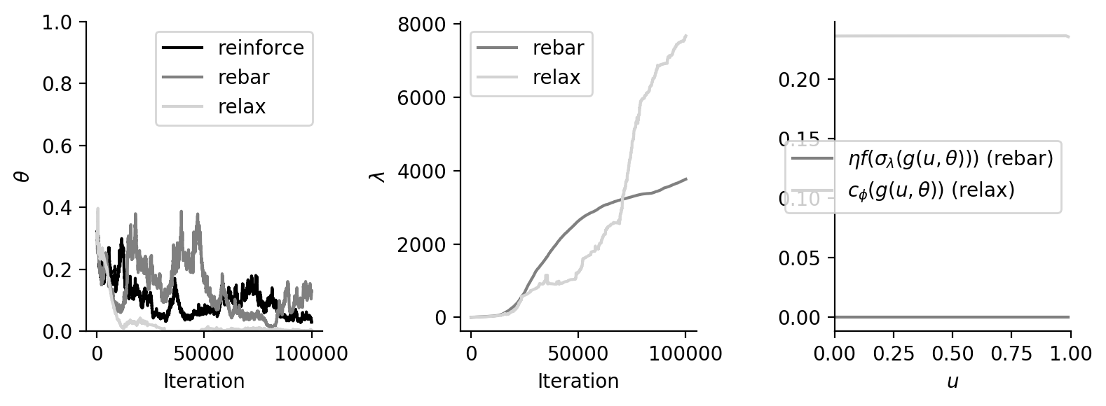
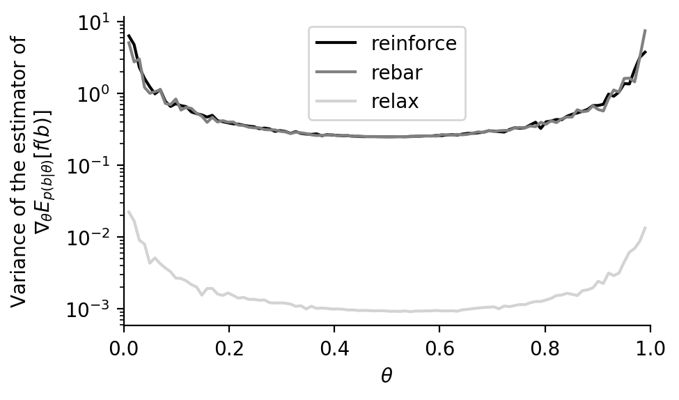
Experiments

Let \(f(b) = (b - t)^2\) where \(t = 0.499\). This results in a difficult estimation problem because the true gradient \(g = 1 - 2t\) is \(0.02\) in this case. If the variance is too high, we won’t be able to move in the right direction.

In the Rebar case, we use \begin{align} c_{\phi}^{\text{rebar}}(z) = \eta f(\sigma_\lambda(z)) \end{align} where \(\phi = (\eta, \lambda)\) and \(\sigma_\lambda(z) := (1 + \exp(-z / \lambda))^{-1}\) is the inverse logit or logistic function.

In the Relax case, we use \begin{align} c_{\phi}^{\text{relax}}(z) = f(\sigma_\lambda(z)) + r_\rho(z) \end{align} where \(\phi = (\lambda, \rho)\) where \(r_\rho\) is a multilayer perceptron with the architecture [Linear(1, 5), ReLU, Linear(5, 5), ReLU, Linear(5, 1), ReLU] and the weights \(\rho\).

Optimization and variance of the estimator with the final \(c_\phi\) (doesn’t work yet):

[back]